


This page explains what the coherency, phase and gain functions are and how the customer can use them. This page describs a part of the data analysis services we offer at CRI. Please click "Data Analysis" button above to see other types of data analysis we offer.
We prepared explanatory pages with some examples for underlined words in blue. If you want to see those pages, please click underlined words in blue below.
What are coherency function, phase function and gain function?
Coherency function shows the degree how much two sets of time series are resembled each other by numbers ranging from 0(not resembled at all) to 1(perfectly resembled). The advantage of coherency function over correlation coefficient is that Coherency function is a function of frequency. In other word, it can show that at which frequencies two sets of time series data are coherent and at which frequencies they are not. Numerically, one might interpret coherency function as a cross spectral density function normalized by the product of power spectral density functions of both time series.
The phase function, which is usually computed with coherency function, shows phase difference as a function of frequency between two sets of time series data. One note about the phase difference is that it is not the same as time difference. For example, if the variations in time series data B are constantly lagged behind those in time series A, say by 2 hours, at all the frequencies, the phase lag at a period of 4 hours is 180 degrees but it is 90 degrees at a period of 8 hours.
The gain factor of the frequency response function shows the amplitude relationship between two sets of time series data as a function of frequency. The gain factor combined with coherency function and phase function would give us fairy clear picture about the relationships between two sets of time series data if they have common variations. We think that correlation coefficient is not that much useful if time lag of coherent variations between two sets of time series data is different at different frequencies. The caveat here is that, even if coherency function indicates there are common variations, they might be utterly unimportant because the amplitudes of those variations might be rather minuscule. It is still necessary to look at a power spectral density function of, at least, one of the time series data to know the amplitude of those coherent variations for this reason. Also, we implicitly assume that the processes at work are linear (output is proportional to input) when we use these functions to analyze data. We can evaluate confidence interval of these functions similar to those of spectral density functions. The computations of coherency function, phase function and gain factor are not any more expensive than computation of a simple correlation coefficient at CRInternational.
What do coherency function, phase function and gain function of actual data look like?
Figure 1 shows time series plots of east-west (zonal) current at 0S-156E and at 0S-165E (on the equator) at the depth of 100m (328 feet or 54.6 fathom). These data are obtained from National Oceanic and Atmospheric Administration, U.S.A.( http://www.pmel.noaa.gov/tao/).
Announcement
We started offering low cost micro-job style computational services. For more information, please click
->here<-.
please send a mail
-->here<--
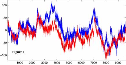
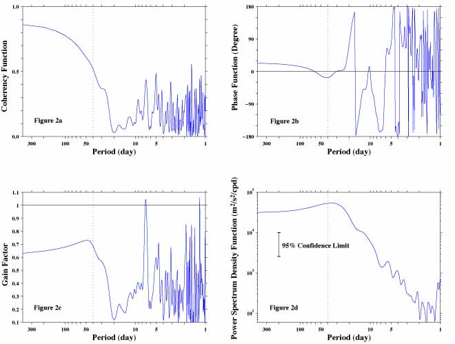
Figure 2a shows coherency function. The coherency is over 0.8 at long periods (low frequency) but it starts dropping rather fast as period decreases. It becomes 0.5 at about 40-day period (dotted black vertical line) and it hits floor at about 20-day period. From there it changes rapidly but stays low as period further decreases. Thus, coherency function shows what appears to be highly correlated these two sets of time series are actually highly coherent only at period longer than about one month.
Figure 2b shows phase function and horizontal black line indicates 0 degree (no phase/time lag between these data). The phase changes the sign within a range where the coherency is high. This means that the variations of current at 156E lagged behind those at 165E at very long periods but the order changes at about 60-day period. However, the phase at period longer than about 25-day is not statistically significantly different from zero.
The gain factor, figure 2c shows that the amplitude of variations at 165E is smaller than that at 156E at almost entire period range (values are less than 1.0). There is a slight tendency that amplitude of variations at 165E relative to that at 156E increases as period decreases within a range where coherency is high.
Finally, figure 2d shows power spectral density function of the current at 156E. It is noted that there are relatively strong energy at periods shorter than 40-day period. This suggests that those variations at periods where the coherency was low are not negligible.
We hope, this example shows how useful coherency and other related functions are.
We would like to mention that the coherence between the current at 156E and at 165E at long periods is unusually high considering the distance between these two position is about 1000km(about 540 nautical miles and 625 land miles). This is a characteristic of near surface current on the equator. If you are interested in this topic, please click here or see the site (NOAA/PMEL) where we downloaded these data.
Is coherency function always useful?
Yes and no. Since coherency function is computed from cross spectral density function and power spectral density functions, same cautions described in the explanation of power spectral density function are necessary.
What can I do if I have more than three sets of time series data and want to analyze the relationships among them?
Let say you have one set of time series data which represents output and 9 other sets of time series data that are input and you want to see the relationships between input and output. You can have 9 sets of figures of coherency function, phase function, gain factor and power spectral density function, place them on your desk and see how they look like. They might occupy entire surface of your desk but we think you can do it. You might be able to condense your figures into one for each function by drawing contours of isopleths. Then, there might be a case when you want to know the common variations amng all of those 10 sets of time series data and want to treat all of them equally. What can you do to analyze the relationships among them? There are 45 combinations of picking up 2 sets of data out of 10 sets of them. We think it is a bit of hassle to place 45 sets of figure on a desk and try to see them all. Instead, we recommend you to apply an Empirical Orthogonal Function (EOF) analysis, which is basically a principle component analysis applied to time series data. The EOF analysis has been used by earth scientists for over 20 years and has made some significant contributions.